Working with RNA-seq data
Data Carpentry contributors
Learning Objectives
- Recall principles of data tidiness
- Use dplyr to explore RNA-seq data
- Use the split-apply-combine principles to summarise RNA-seq data
- Make plots with ggplot2 to explore expression changes in an RNA-seq timecourse.
Reading in the RNA-seq data
In this lesson we’re going to use a published RNA-seq dataset to show how the concepts and tools from previous lessons can be applied to genomic data. The data comes fom Jeong et al., 2017 (https://www.nature.com/articles/s41467-017-00738-7) and is a summary of RNA-seq data from the mouse retina at several different timepoints. HTSeq was used to count the number of reads from each RNA-seq dataset aligning to each mouse gene, which were normalised for differences between libraries using the TMM method from the edgeR package (Thanks to Benjamín Hernández Rodríguez for providing the prepared data!).
First let’s read in the prepared data and create a data frame.
expression_df <- read.table("expression_data.tsv", sep = "\t", header = TRUE)
head(expression_df)
## ensembl_gene_id timepoint replicate norm_counts
## 1 ENSMUSG00000000001 P6 1 384.45093
## 2 ENSMUSG00000000003 P6 1 0.00000
## 3 ENSMUSG00000000028 P6 1 38.09874
## 4 ENSMUSG00000000031 P6 1 130.45933
## 5 ENSMUSG00000000037 P6 1 34.63522
## 6 ENSMUSG00000000049 P6 1 0.00000Challenge
With a partner, discuss the data tidiness principles from yesterday and write the ones you can remember in the etherpad.
Challenge
Take a look at the RNA-seq dataset. What data does each column hold? Does this data frame follow the data tidiness principles? Hint: the
summaryfunction might be useful here.
This dataset follows the data tidiness principles from the data organisation lesson: each column contains a different variable and each row is a different observation.
Data exploration
Challenge
How many different timepoints are there in this dataset? How many different replicates are there for each timepoint?
table(expression_df$replicate, expression_df$timepoint)##
## P10 P15 P21 P50 P6
## 1 39179 39179 39179 39179 39179
## 2 39179 39179 39179 39179 39179
## 3 39179 39179 39179 39179 39179There are five different timepoints with three replicates each.
How much variability is there between replicates? Let’s make some plots to see, but we’ll just use a subset of the data. We can use filter to select a subset of the data.
genes_sub <- expression_df$ensembl_gene_id[1:10]

counts_sub <- filter(expression_df, ensembl_gene_id %in% genes_sub)

ggplot(counts_sub, aes(x = ensembl_gene_id, y = norm_counts, colour = timepoint, shape = as.character(replicate))) +
geom_point() 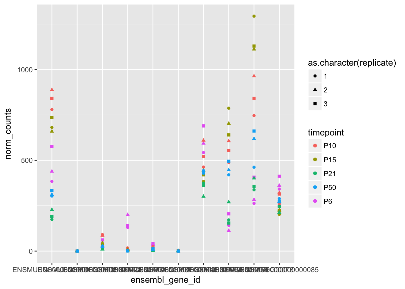
The three replicates at each timepoint look pretty close for all these genes, so let’s assume that there’s no systematic biases between the three replicates. There are better ways to check if there are biases or batch effects in your RNA-seq data, like performing a Principal Component Analysis, but we don’t have time to cover that here.
Summarising data
Remember the split-apply-combine concept from the dplyr lesson? We can apply that here to get the average expression for each gene at each timepoint. Here we’re splitting the data into groups based on the gene ID and timepoint, then summarising each group by taking the mean of the counts and putting it in a new column.
summary_df <- expression_df %>%
  group_by(ensembl_gene_id, timepoint) %>%
  summarise(mean_counts = mean(norm_counts))
Combining datasets
It would be helpful to know some more information about these genes, such as the gene names, which are more recognizable to humans than the gene IDs. We can read in another table of data about the genes and combine it with the expression data.
genes_df <- read.table("gene_data.tsv", sep = "\t", header = TRUE)
head(genes_df)
## ensembl_gene_id gene_name gene_biotype exons_width_bp cluster
## 1 ENSMUSG00000000001 Gnai3 protein_coding 3262 5
## 2 ENSMUSG00000000003 Pbsn protein_coding 1599 NA
## 3 ENSMUSG00000000028 Cdc45 protein_coding 4722 4
## 4 ENSMUSG00000000031 H19 lincRNA 6343 1
## 5 ENSMUSG00000000037 Scml2 protein_coding 23080 1
## 6 ENSMUSG00000000049 Apoh protein_coding 2662 NAThis new dataset tells us the ID and name for each gene, the type of gene, and the total size of the gene’s exons. We’ll come back to the “cluster” column later. We can use the “join” family of functions from dplyr to combine datasets.
combined_df <- left_join(summary_df, genes_df, by = "ensembl_gene_id")
head(combined_df)
## # A tibble: 6 x 7
## # Groups: ensembl_gene_id [2]
## ensembl_gene_id timepoint mean_counts gene_name gene_biotype
## <fctr> <fctr> <dbl> <fctr> <fctr>
## 1 ENSMUSG00000000001 P10 836.3700 Gnai3 protein_coding
## 2 ENSMUSG00000000001 P15 691.8978 Gnai3 protein_coding
## 3 ENSMUSG00000000001 P21 198.0894 Gnai3 protein_coding
## 4 ENSMUSG00000000001 P50 315.8944 Gnai3 protein_coding
## 5 ENSMUSG00000000001 P6 466.2814 Gnai3 protein_coding
## 6 ENSMUSG00000000003 P10 0.0000 Pbsn protein_coding
## # ... with 2 more variables: exons_width_bp <int>, cluster <int>For this lesson, we’re only interested in protein coding genes, so let’s subset the data to remove other gene biotypes. First, what gene biotypes are in this dataset?
table(combined_df$gene_biotype)##
## 3prime_overlapping_ncrna antisense IG_C_gene
## 5 7380 65
## IG_D_gene IG_J_gene IG_LV_gene
## 125 440 1520
## IG_V_gene IG_V_pseudogene lincRNA
## 10 5 8975
## miRNA misc_RNA Mt_rRNA
## 10050 2960 10
## Mt_tRNA polymorphic_pseudogene processed_transcript
## 110 75 3530
## protein_coding pseudogene rRNA
## 113700 29725 1765
## sense_intronic sense_overlapping snoRNA
## 450 50 7780
## snRNA TR_V_gene TR_V_pseudogene
## 6935 225 5Most genes are protein coding but there are many other gene biotypes present.
filtered_df <- filter(combined_df, gene_biotype == "protein_coding")
table(filtered_df$gene_biotype)
##
## 3prime_overlapping_ncrna antisense IG_C_gene
## 0 0 0
## IG_D_gene IG_J_gene IG_LV_gene
## 0 0 0
## IG_V_gene IG_V_pseudogene lincRNA
## 0 0 0
## miRNA misc_RNA Mt_rRNA
## 0 0 0
## Mt_tRNA polymorphic_pseudogene processed_transcript
## 0 0 0
## protein_coding pseudogene rRNA
## 113700 0 0
## sense_intronic sense_overlapping snoRNA
## 0 0 0
## snRNA TR_V_gene TR_V_pseudogene
## 0 0 0Plotting the data with ggplot2
We can plot the results with the ggplot2 package to see what the overall gene expression pattern looks like over time.
ggplot(filtered_df, aes(x = timepoint, y = mean_counts)) +
  geom_boxplot() +
  scale_y_log10()
## Warning: Transformation introduced infinite values in continuous y-axis## Warning: Removed 31430 rows containing non-finite values (stat_boxplot).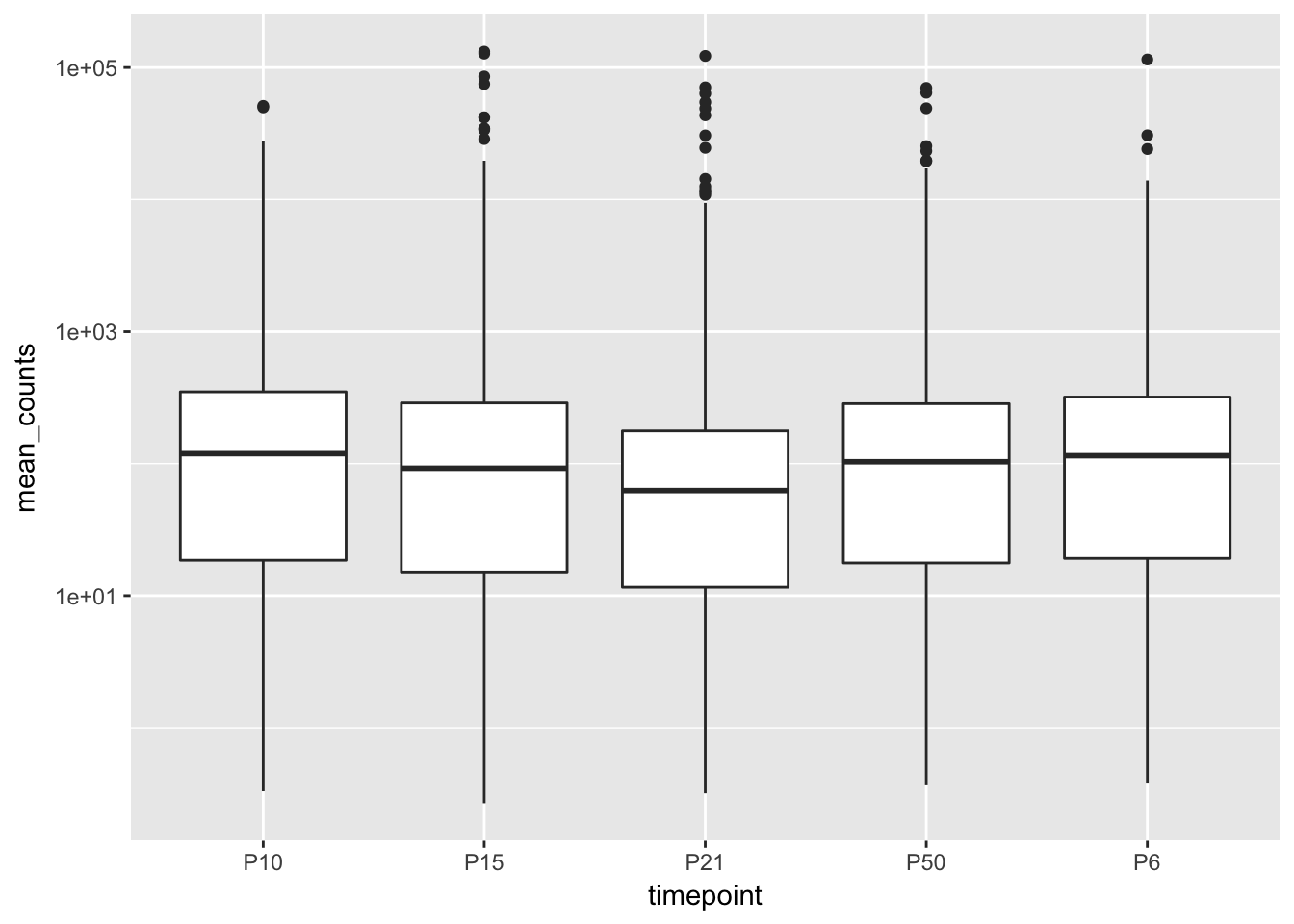
Notice the order of the x axis. This is sorted alphabetically, which doesn’t give us the right order in time. The “timepoint” column is a factor, and the levels of the factor are by default sorted alphabetically, but we can change that by manually specifying the order we want the levels to be in. To do this, we can use the “mutate” function from dplyr.
filtered_df <- mutate(filtered_df, timepoint = factor(timepoint, levels = c("P6", "P10", "P15", "P21", "P50")))

ggplot(filtered_df, aes(x = timepoint, y = mean_counts)) +
  geom_boxplot() +
  scale_y_log10()
## Warning: Transformation introduced infinite values in continuous y-axis## Warning: Removed 31430 rows containing non-finite values (stat_boxplot).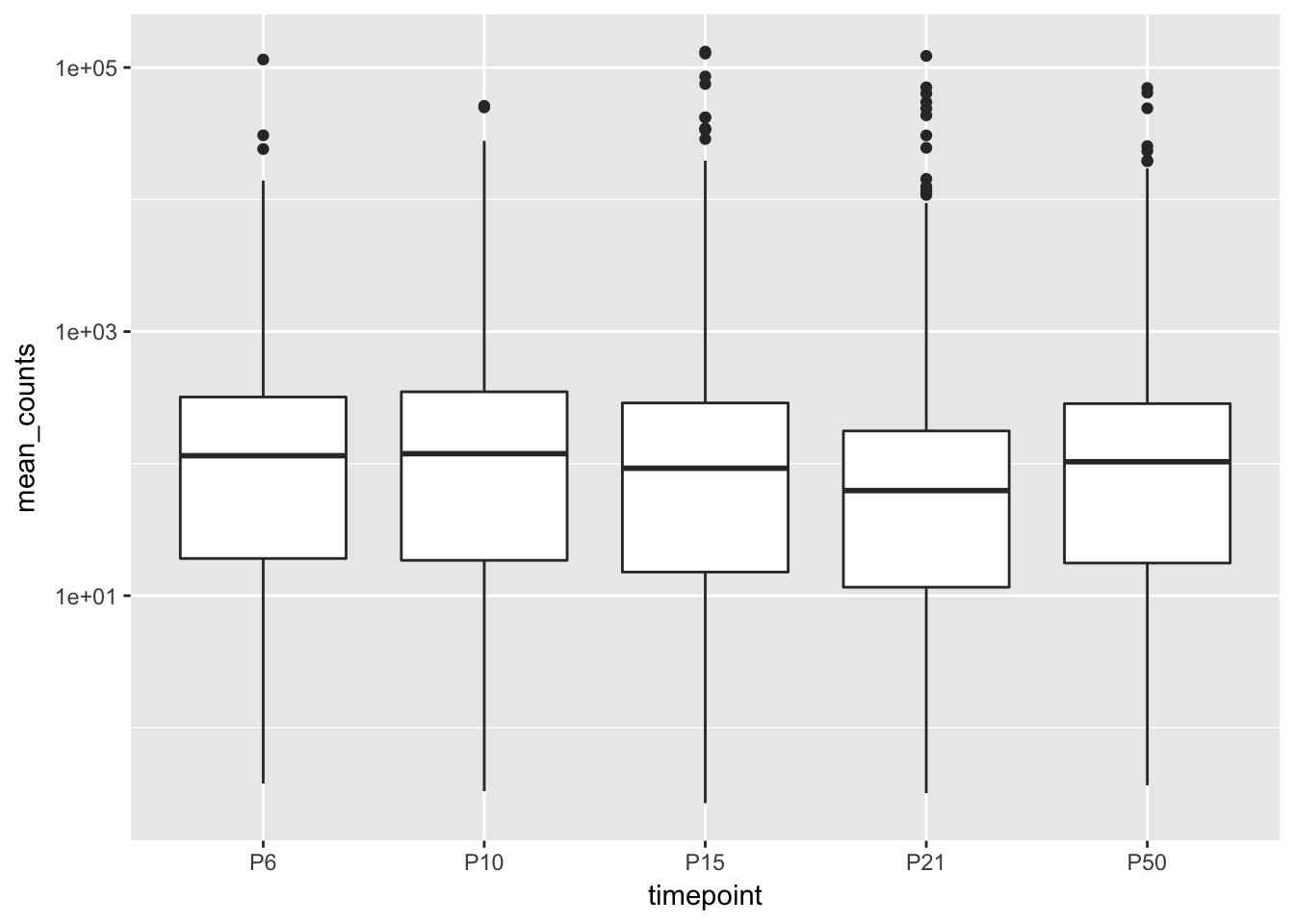
That’s better!
More data exploration
In order to more easily compare expression between different genes, it’s often useful to calculate expression normalised by gene length. In papers you often see “TPM” (transcripts per million reads) or “FPKM” (fragments per kilobase per million reads), which also normalise for the number of mapped reads. Calculating those is a bit more complicated, and you can read more about it (here)[https://haroldpimentel.wordpress.com/2014/05/08/what-the-fpkm-a-review-rna-seq-expression-units/]. Important: these measures should only be used for comparing relative gene expression within a sample, or for visualisation. Use raw counts for doing differential expression analysis.
Challenge
Calculate expression normalised by gene length in kilobases, using the “norm_counts” and “exons_width_bp” columns, and add this to the dataset as a new column, using the
mutatefunction.
filtered_df <- mutate(filtered_df, expr_per_kb = mean_counts / (exons_width_bp / 1000) )Using the expression normalised by the gene length, we can safely compare between genes in the same sample. For example, which genes have the highest expression at P6?
max_p6 <- filtered_df %>%
  filter(timepoint == "P6") %>%
  ungroup() %>%
  top_n(n = 10, wt = expr_per_kb)

max_p6
## # A tibble: 10 x 8
## ensembl_gene_id timepoint mean_counts gene_name gene_biotype
## <fctr> <fctr> <dbl> <fctr> <fctr>
## 1 ENSMUSG00000001270 P6 5542.269 Ckb protein_coding
## 2 ENSMUSG00000029580 P6 24142.555 Actb protein_coding
## 3 ENSMUSG00000034994 P6 6894.143 Eef2 protein_coding
## 4 ENSMUSG00000049775 P6 6378.523 Tmsb4x protein_coding
## 5 ENSMUSG00000056201 P6 3186.404 Cfl1 protein_coding
## 6 ENSMUSG00000064351 P6 30668.318 mt-Co1 protein_coding
## 7 ENSMUSG00000064354 P6 2774.148 mt-Co2 protein_coding
## 8 ENSMUSG00000064357 P6 1781.325 mt-Atp6 protein_coding
## 9 ENSMUSG00000064358 P6 7664.456 mt-Co3 protein_coding
## 10 ENSMUSG00000064360 P6 2474.227 mt-Nd3 protein_coding
## # ... with 3 more variables: exons_width_bp <int>, cluster <int>,
## # expr_per_kb <dbl>What about the gene from each cluster with the highest expression at this timepoint? Using the group_by function before top_n will return the top genes from each group.
max_p6 <- filtered_df %>%
  filter(timepoint == "P6") %>%
  group_by(cluster) %>%
  top_n(n = 1, wt = expr_per_kb)

max_p6
## # A tibble: 8 x 8
## # Groups: cluster [8]
## ensembl_gene_id timepoint mean_counts gene_name gene_biotype
## <fctr> <fctr> <dbl> <fctr> <fctr>
## 1 ENSMUSG00000001270 P6 5542.2691 Ckb protein_coding
## 2 ENSMUSG00000025982 P6 7564.2635 Sf3b1 protein_coding
## 3 ENSMUSG00000029580 P6 24142.5547 Actb protein_coding
## 4 ENSMUSG00000036905 P6 1994.6925 C1qb protein_coding
## 5 ENSMUSG00000049775 P6 6378.5233 Tmsb4x protein_coding
## 6 ENSMUSG00000050621 P6 445.0116 Gm9846 protein_coding
## 7 ENSMUSG00000060802 P6 1565.4474 B2m protein_coding
## 8 ENSMUSG00000064351 P6 30668.3176 mt-Co1 protein_coding
## # ... with 3 more variables: exons_width_bp <int>, cluster <int>,
## # expr_per_kb <dbl>What are the expression patterns of these genes over the timecourse?
Challenge
Filter the filtered_df data frame to contain only rows referring to the genes with the highest expression in each cluster at P6. Make a plot to show how the expression of these genes changes over time.
filtered_df %>%
  filter(gene_name %in% max_p6$gene_name) %>%
  ggplot(aes(x = timepoint, y = expr_per_kb, colour = gene_name)) +
  geom_line(aes(group = gene_name)) +
  geom_point() +
  facet_wrap(~cluster, scales = "free_y")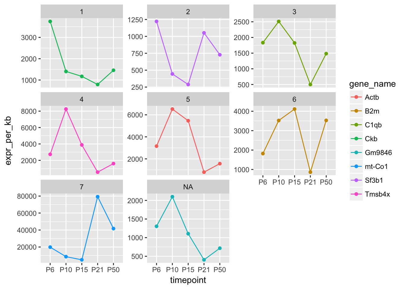
Extra challenges
Challenge
Repeat the analysis above with the top ten genes with the highest expression at P6.
Challenge
Repeat the analysis above with the genes with the highest expression at a different timepoint.
Challenge
Customise your plots!
Data Carpentry,
2017. License. Contributing.
Questions? Feedback?
Please file
an issue on GitHub.
On
Twitter: @datacarpentry